 |
| Tested Coax Cable Samples |
Greg Ordy
Almost 5 years ago I put together a web page that presented data showing that the Bury-Flex samples I had at my house presented a 45 Ohm characteristic impedance, as opposed to the stated and standard 50 Ohms. In the spring of 2010, I was contributing to an antenna project down in Florida that consisted of a 4-band vertical antenna. As part of that project, I met up with Wil, K1MIJ. In the conversation that surrounded that project, we started to talk about coaxial cables, and I mentioned my 2005 results. Since Wil had Bury-Flex available at his station, he was curious to know if the situation had changed. I admit I was also wondering, so he sent me a few feet of sample cable, and I set out to remake the 2005 measurements. The samples he sent me were purchased less than 2 years ago (2008 time frame).
This page describes those measurements and results.
For those that can't wait for the end of the story, the impedance of the more recent Bury-Flex I measured is 50 Ohms.
I installed several hundred feet of Bury-Flex at the end of the last century - the 1990's. I picked the cable because of its low loss specification, and the ability to directly bury it. I have two major runs, each over two hundred feet long, that radiate out from the house in separate directions to two antenna fields. I also used the cable on my tower, and around the rotator, using the Flex part of Bury-Flex.
As you might be able to tell from my other web pages, I enjoy experimenting with antennas, and sooner or later that gets into the measurement of SWR, impedance, and other antenna parameters. Usually I make measurements directly at the antenna, and expect that the conditions in the station can be assumed given the properties of lossy transmission lines. One day, when I was more carefully measuring antennas inside and outside of the station, I noticed that SWR readings inside the station were sometimes higher than at the antenna. This is a rather odd situation, since with ideal lines the SWR is constant, and not a function of the line length, and, with real world lossy lines, the effect of line loss is to lower the SWR, not raise it. These comments assume that the radio (SWR measurement device) and line are the same impedance, let's say 50 Ohms.
How could this be? The loss on my cables should be knocking down the SWR a bit, not raising it. After some head scratching, I ended up measuring some spare cable from the cabinet, and it measured close to 45 Ohms, not 50 Ohms. This explained everything.
Let's say I had an antenna that was a perfect 50 Ohms resistive at the antenna feed point. It could be a dummy load. With 50 Ohm cable, the impedance would stay at 50 Ohms at the station side, which is still an SWR of 1. If, however, the cable impedance was 45 Ohms, and, the cable happened to be 1/4 wavelength long, the transformer action on the mismatched line would present an input impedance of 40.5 Ohms. Relative to a 50 Ohm system, the radio, the SWR would now be 50/40.5 = 1.23. So, that is an example where the 45 Ohm cable could increase the SWR; 1.0 at the antenna becomes 1.23 at the radio. It is also possible to create examples where the cable could improve the match. While impedance matching with carefully calculated transmission line lengths (series matching sections) is a great technique, I wasn't looking for this property in my general purpose multiple band feed lines!
I should mention that other than this property, everything else about the cables met and exceeded the specifications and my needs. To this day, all contacts I make are still over buried Bury-Flex. The cable has been in service over 10 years, and it appears in good shape. The flex properties around the rotator were excellent. I replaced the cable with other popular flexible cables, and I had to replace them when they self-destructed after a year of use.
A good question to ask is: how representative of all Bury-Flex were the cables I tested? My recollection is that I purchased two multiple hundred foot spools of Bury-Flex separated in time by a year or two. Both batches tested the same way. You can form your own opinion.
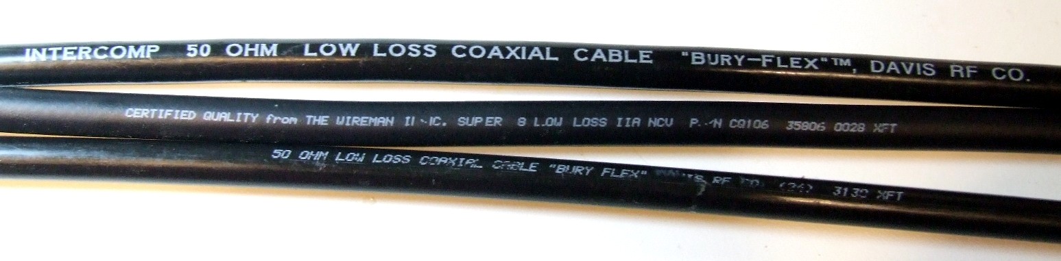
To be crystal clear, I'm talking about Bury-Flex made by Davis RF, also known as 9914F.
The cables that Wil sent me were approximately 6 feet long. I went into my coax cabinet and found a piece of my original Bury-Flex that was similar in length. I should mention that Wil also sent me a sample of The Wireman Super 8 cable. This is a line that is similar to Bury-Flex. I installed PL-259s on each end to aid in quick and repeatable changing. For the record, the lengths of the three examples were as follows:
| Cable | Length |
| Original Bury-Flex | 99 inches |
| Wireman Super 8 | 62 inches |
| Recent Bury-Flex | 73 inches |
Here is a picture of the three cables. Note that the labeling of the Bury-Flex changed over the years (the original cable is the top one). Please click on the picture for a larger view.
|
|
| Tested Coax Cable Samples |
There are probably many different ways to measure the characteristic (or surge) impedance of a coaxial transmission line cable. 5 years ago, on the original web page, I used a technique where I terminated a section of cable with a resistive load, and swept a range of frequencies while recording the complex impedance. The results were then plotted on a Smith Chart, revealing the Zo (characteristic impedance) of the cable. This is a simple and effective method, and it will give me a chance to launch into some Smith Chart discussion.
A second method is far more accurate, and I have used it many times in recent years. That method will also be used.
Let's say that you terminate any length of transmission line with an impedance equal to its characteristic impedance. At any frequency, the measured impedance will be that same impedance. A 50 Ohm line, terminated with a 50 Ohm load, measures as 50 Ohms at all frequencies. This condition has been called a nonresonant line. What is the SWR caused by the 50 Ohm load? Since the load impedance equals the line impedance, there is no mismatch, and the SWR is 1.
Let's now change the load impedance to a 100 resistor, that is, a pure resistance, no reactance. Let's also get rid of the transmission line so that if we ask what the impedance of the load is we can easily answer 100 Ohms - that's all we have, a 100 Ohm resistor with a pile of 50 Ohm coax lying in the corner. Let's plot that on a Smith Chart, keeping in mind that we are going to quickly introduce a 50 Ohm transmission line. I have chosen to zoom in to the inner regions of the chart so that it's easier to read and follow.
 |
| 50 Ohm Smith Chart with a 100 + j0 Impedance Plotted |
Because we will be focused on the effects of a 50 Ohm transmission line, we make that value, 50 Ohms, the Prime Center of the Smith Chart. We then will normalize to 50 Ohms, meaning that all resistance and reactance values we want to work with must be divided by 50 before we can place them on the chart. And, when we take a value off of the chart, we have to reverse the process, and multiply by 50 Ohms to get to real values.
The red point is drawn on a horizontal axis line where we see the value 2.0. That's because 2.0 X 50 = 100. There is no reactance present, so we lie right on the resistance axis that runs from left to right through the center of the Smith Chart circle.
Now I must confess that I am going to gloss over the details of plotting impedance points. There are many web sites with good information and tutorials on the topic. Just trust me that I'm going to put the points close to the right place.
I now go to corner of the room and pick up a pile of coax jumpers, each 10 degrees long. By working in units of degrees I can be independent of frequency, so long as the frequency is fixed. But, if that's a conceptual problem, let's say that the frequency is 7 MHz, and because the velocity factor of the cable is 0.66, each 10 degree segment is the same as 2.576 feet of cable. I hook up 10 degrees of cable and measure the complex impedance at the input to the cable with the 100 Ohm resistor at the end. I add 10 more degrees and measure again. I keep doing this in increments of 10 degrees through 60 degrees. What values did I write down? While I'm at it, I'll compute the normalized values of the impedance. These are just the measured R and X values divided by 50.
| Degrees | R (Resistance) | X (Reactance) | Normalized R | Normalized X |
| 10 | 91.70 | -23.53 | 1.83 | -0.47 |
| 20 | 74.02 | -35.69 | 1.48 | -0.71 |
| 30 | 57.14 | -37.12 | 1.14 | -0.74 |
| 40 | 44.65 | -32.98 | 0.89 | -0.66 |
| 50 | 36.23 | -26.76 | 0.72 | -0.54 |
| 60 | 30.77 | -19.99 | 0.62 | -0.40 |
Now by just looking at the data, can we see any sort of trend or pattern that would seem to make sense with the fact that we are going from point to point by adding a constant length of cable? To me, I can't see anything exciting, this is a big mess if you ask me. I guess that the resistance is dropping, and maybe that's a pattern, but the reactance peaks to around -37 Ohms and then starts going in the other direction. What's up with that?
Ok, let's plot those points on the Smith Chart. That means plotting the normalized values, that's why I had to compute them in the table - I needed them.
 |
| 100 + j 0 Through 10 Degree Increments of Transmission Line |
Hopefully it's obvious that the shape we are drawing is a circle centered on the center of the Smith Chart, and with a radius that is equal to the 100 + j 0 Ohm point. Ok, let's assume that if we kept adding 10 degree sections of cable we would complete the circle. Let's just draw the darn circle.
 |
| SWR 2.0 Circle |
Let's not miss any fine points. We started with no cable and 100 Ohms. We plotted that point, and then started to add cable which added points. We ended up on a circle over the center of the chart. The points we added went clockwise around the circle as we added more cable. 60 degrees of points covered the bottom 2/3 of the circle. That means that 90 degrees, or 1/4 wavelength, would cross the resistance axis at 0.5, which means 0.5 X 50 = 25 Ohms. This is the action of the famous 1/4 wavelength transformer. We took a 100 Ohm resistor, and by putting 1/4 wavelength of 50 Ohm cable in front of it, we have created a 25 Ohm resistor - at that single frequency. Since the idea of frequency dependent resistors is rather odd, it's more comfortable to start to talk about impedance. If we add 90 more degrees of cable, we get back to our starting point. That's why folks have said that you can accurately measure impedance (at one frequency) through a 1/2 wavelength section of cable. It's clear that any other length would transform the impedance. Of course if you knew how long a given cable was, you could use the Smith Chart, working counterclockwise, to figure out the impedance at the load end of the cable, by undoing the effect of the transmission line. It's just a matter of moving the correct angular distance along a circle.
Perhaps the most interesting aspect of the points that lie on the circle is that their impedance values, although different, have the same SWR. When you draw a centered circle on the Smith Chart, you are creating a set of impedance values with the same SWR, and the SWR is a function of the length of the radius. For example, both 100 Ohms and 25 Ohms present a 2 to 1 SWR to a 50 Ohm reference.
The important concept to take away from that observation is that transmission lines cause impedance values to change, but the SWR remains constant, and is not a function of line length. If you are trying to measure the impedance of something, and a transmission line is between you and that something, that line will shift the impedance readings. SWR, however, will not be affected.
In the real world, the amount of cable loss does alter the result. Loss causes perfect circles to become spirals that slowly spiral towards the center of the chart. Loss sucks.
Now I need to mention the one bait-and-switch trick that I'm about to pull. In the previous example, we had this nice supply of transmission line sections that we could join together to make longer and longer cables. How often does that happen in the real world? We can certainly care about the length of a transmission line when we are using it for impedance matching purposes, but that's not the same as having a box full of uniform sections that we join together. What is far more common is to change the frequency while keeping the line length fixed. Changing the measurement frequency on a fixed line length is very similar in effect to changing the length of a line with a fixed frequency. For example, a line that is 25 degrees long at 7 MHz will be 50 degrees long at 14 MHz. It's the same physical line, but when we change frequency we change the number of degrees that length represents. So, rather than needing a huge box of small transmission line segments that we can use to make lines of any length, we can observe the same phenomena by keeping the line length constant and changing frequency. There are some differences between the two, but we are usually working with fixed line lengths and measurement devices/radios that can change frequency, so that's the far more common situation.
What if rather than a 100 Ohm load I would have used a 50 Ohm load? Since that's a perfect match, the circle would collapse to a point in the center. If you want, consider a point to be a circle with a really small radius. What if I would have used a 200 Ohm resistor? In that case, the radius of the circle would be larger, starting at the value of 4, since 200 / 50 = 4. What about the value when I add a 1/4 wavelength of cable? With 100 Ohms we created 25. But, with 200 Ohms we rotate around the halfway circle to create 12.5 Ohms. Since the radius of the circle has changed, the SWR has also changed. The SWR is 4, whether the load is 200 Ohms, 12.5 Ohms, or any other value on the same circle.
Ok, let's get radical. What happens if we used a 300 Ohm transmission line with a 400 Ohm load? With a zero length line, the impedance would be 400, and the SWR = 400 / 300 = 1.333. If we added 1/4 wavelength of 300 Ohm cable, the SWR would remain the same, but the impedance would rotate around the chart to 300 / 1.333 = 225 Ohms. If we moved the center of the Smith Chart to 300 Ohms as opposed to 50, we know that the 400 and 225 Ohms would create a perfectly round centered circle. But what happens if we leave the Smith Chart as a 50 Ohm chart, and add the 300 Ohm data? We have 3 data points to consider, 225, 300, and 400 Ohms. If we want to draw them on a 50 Ohm Smith Chart we have to normalize by 50, creating the values of 4.5, 6, and 8. Let's plot those, and see if we can draw a circle centered on 6, the 300 Ohm value that represents our cable Zo.
 |
| 300 Ohm Data Plotted on a 50 Ohm Smith Chart |
I know it's a little hard to see, but I did attempt to faithfully drop colored circles on the values of 4.5, 6, and 8. And, the distance from 4.5 to 6 is the same as from 6 to 8. Obviously the axis is not linear. Since the radial distance is the same, we can indeed draw a round circle.
The purpose of this exercise is to show that even though we have a 50 Ohm Smith Chart, the impact of rotating an impedance through a 300 Ohm cable still appears as a circle. The center of the circle is shifted to impedance of the cable. For many operations on a Smith Chart, willy-nilly mixing of different system impedances creates issues. But, this is a case where we can combine data onto one chart.
This also motivates the method I used 5 years ago to claim that the Bury-Flex I had was a 45 Ohm cable. We have now seen that if we take a load and connect it to a cable, and measure the cable input impedance as we shift frequency (or length), and then plot those impedance points, we will create a circle that is centered on the cable's Zo. If we happen to pick a load that is the same impedance as the cable we will have a point, not a circle.
The measurement approach is as follows:
Select a load impedance. Often times we have lying around 50 or 75 Ohm loads, even a 1000 watt dummy load is fine.
Connect the load to the unknown cable. Based upon your measurement device, sweep a reasonable frequency range recording the input impedance.
Plot the impedance on a Smith Chart.
If you happened to pick a load impedance that is the same as the cable impedance, you will see a very small and tight circle or spiral.
Otherwise, you will draw a circle. The center of the circle is the cable impedance.
The length of the test cable and the sweep range will determine how much of a circle you draw. If you have a very short arc, determining the center of the implied circle could be very difficult.
For the 3 cables I'm measuring this time around, I connected each to the same 50 Ohm load and swept the frequency from 1 through 50 MHz. The resulting graph was:
 |
| Cable Comparison |
The red and blue traces are the Super 8 and new Bury-Flex cables. They start off as a tight spiral right at the center of the chart, which is 50 Ohms. This is also the 1 MHz end of the trace. I believe that the movement out of the center at higher frequencies is due to my poor 50 Ohm load, where I used 2 adapters to connect the load to the cable. Being UHF series plumbing, they are not constant impedance, and as the frequency rises, this will cause the load to become more reactive.
The green trace is the old Bury-Flex. This traces does start off very close to 50 Ohms at 1 MHz. That's because as the frequency drops, with a short cable, the transmission line behavior becomes less, and at DC we would only measure the 50 Ohm load. As the frequency rises, however, we see the circle/spiral clearly center around 0.9, which we multiply by 50 to convert into 45 Ohms.
If you are not looking at the impedance data on a Smith Chart, then you are probably looking at it plotted on a typical rectangular graph. Here is the same data plotted that way.
 |
| Rectangular Graph Cable Comparison |
The resistance values are clustered up near 50, and the reactance is down near zero. It's obvious that one of the three cables is different than the other two. What isn't so clear is the signature of being a 45 Ohm cable with an 50 Ohm load. Perhaps the cable was crushed, or water logged, or even packed in liquid Boron. Here's where the Smith Chart helps suggest what's really going on.
In recent years, I became aware of a technique to compute the complex Zo of a transmission line based upon the measurement of the complex cable input impedance with an open and then a shorted load. The formula is:
 |
| Formula for Computing Transmission Line Zo (from Chipman) |
This formula works at any frequency, and within reason with any line length. I have adopted the following test procedure, and used it many times with a wide range of cables.
Connect the load end of the test cable to an open circuit. Sweep and record the complex impedance from 1 through 50 MHz in steps of 100 KHz.
Connect the load end of the test cable to a short circuit. Sweep and record the complex impedance from 1 through 50 MHz in steps of 100 KHz.
Transfer the pairs of R and X values to an Excel spreadsheet that I seem to always reuse for this purpose. The spreadsheet implements the previous formula. The only trick is understanding that Excel operates on complex data using special functions that might need to be loaded from a library.
Graph the R and X components of Zo. Perform a sanity check on the graph, checking for gross data capture and/or transcription errors.
Compute the average R and X values, consider those to be the answer.
The procedure is relatively painless and fast. Mainly, I consider it to be accurate.
Before getting into the numbers, let's talk a little about the history of this formula. I always like to try to find the earliest reference to a formula or solution. Many articles and books, and even web pages, have been written without citing the previous work. Apart from folks potentially being given credit for work that others did, it can be helpful to have references to understand the complete context of the work, and related topics.
In this case, where transmission lines are involved, my two favorite references are:
Transmission Lines, Antennas, and Wave Guides, by King, Mimno, and Wing. This book was published in 1945, and is still an excellent resource.
Transmission Lines, by Robert Chipman (from the Schaum's Outline series). Published in 1968.
The formula appears in Chipman, although King, Mimno, and Wing has all of the parts and analysis that go into the final formula. As best as I can tell, they simply don't put it all together. In many other areas they were out in front. Here's an example. In recent years, the idea of current chokes and antenna currents flowing on the outside surface of a coaxial cable has been a hot topic for discussion. It might seem as if this is some new idea that was relatively recently discovered. Here's what King, Mimno, and Wing have to say about it on page 3 of the book. Remember, this is back in 1945.
 |
| King, Mimno, and Wing Comment on Antenna Currents (page 3) |
For all I know, this might be based upon even earlier work. So, while a book on computers might be out of date 6 months after publication, the old and classic antenna texts still hold up.
Chipman writes the follow on the formula I am using here:
 |
| Transmission Lines, Robert Chipman, Page 134 |
He does go on to caution that you need to be mindful of the limits of your measurement device, especially when the impedance values are close to a parallel resonance. He suggests an odd number of 1/8 wavelengths. Let's see what that means. Here is a graph of the R (red) and X (blue) components of the short measurement of the Super 8 cable.
 |
| Super 8 Cable, Short Load |
What's going on around 37 MHz? At that frequency, the cable, which is only 62" long, is 1/4 wavelength long (an even multiple of 1/8 wavelength). That length transforms the zero Ohm short circuit at the output of the cable to an open circuit or high impedance at the input. It has the shape of a parallel resonant circuit, where the resistance and reactance both rise to a high value, then the reactance shoots through zero to a large negative capacitive reactance, while the resistance drops. I was using a very short cable in this example. There was a single parallel resonance on the shorted end, and none on the open end. This is usually not the case, when test cables are perhaps 10 to 50 feet long. In that case, there can be multiple parallel resonances on both the open and shorted data.
I believe that Chipman would be happy if you simply excluded the data around the wild parallel resonance points, where the rates of change of R and X can be quite high, and the data extremes large. I tend to simply average it all together, since for every positive swing there is eventually a negative swing. In order to get the best results, it is necessary to reduce any changes in length due to applying the open or short load. The frequency and cable length need to be held as constant as possible if you want to get useful data that is close to the parallel resonance points. Slight changes in the cable length between the open and short can create a skew between the data sets. So, the measurement quality matters quite a bit for this computation.
For the data just measured, here is the Zo graph produced by Excel.
 |
| Computed Super 8 Cable Zo |
Averaging the R and X values produces a Zo value for The Wireman Super 8 cable of: 50.50 - j2.42 Ohms. Now we can tell from the data that we have a single negative reactance spike that is going to skew the data in the negative direction. If I scanned to a higher frequency, or, if I had a longer cable, we would include a positive spike that would balance that data out. Given that, we could choose to average the data from a lower range that would certainly cause the reactance to move closer to zero. For example, if we averaged from 5 through 15 MHz, the impedance would be 51.26 - 0.79 Ohms. My preference would be to test a longer cable that would contain several parallel resonance cycles. One thing is for sure. If you can't perform a sweep and ponder the whole data set are we are doing here, make your single measurements near an odd 1/8 wavelength. In this case, the spikes made it through the square root probably because of sloppy measurement technique on my part.
By the way, real coaxial cables do have a small negative reactance in their characteristic impedance. In order to negate that, it would be necessary to artificially add loss to the dielectric, and no cable maker is going to do that.
Here is the Zo graph for the new Bury-Flex cable. In this case, the interaction between the opened and shorted data had less of a speed bump around 32 MHz (don't forget, this cable was 11 inches longer than the Super 8 cable, so the 1/4 wavelength frequency dropped). Note that my measurement technique improved, since the speed bumps are held to a minimum.
 |
| Computed New Bury-Flex Cable Zo |
It's pretty clear by simple inspection that the impedance is close to 50 - j 0 Ohms. The computed average across the range is: 50.13 - j 0.86 Ohms. Let's not get carried away with how accurate these numbers might be. But, to compare against some programs that compute the cable Zo from published data, TLDetails reports a Zo of 50 - j 0.33 Ohms, and the VK1OD calculator reports 50 - j 0.45 Ohms. This is very good agreement between measurements and calculations. It would be helpful if cable makers and sellers published Zo tolerances, so that we could talk about being within specifications, or out of specifications.
Finally, we can apply the same technique to the old Bury-Flex cable.
 |
| Computed Old Bury-Flex Cable Zo |
The averaged Zo value was 45.19 - j0.6 Ohms. As previously claimed, the Zo is close to 45 Ohms.
The data graph shows two blips, one near 23 MHz and the other near 47 MHz. Two blips appear because the old Bury Flex cable is the 99 inches long, which is long enough to show a 1/4 wavelength resonance with the short (23 MHz), and a 1/2 wavelength resonance with the open (47 MHz). Here is a graph of the raw open and short impedance data showing these two resonances.
 |
| Measured Old Bury-Flex Cable Open and Short Response |
To summarize the data and computations, the measured data, representing two complex values and the above shapes, were multiplied together and then the square root was taken. This resulted in the computed Zo graph. The reason why the sharp peaks turn into blips is that the product of the open times the short is relatively constant. This happens when the series and parallel resonances accurately overlap, in some sense averaging each other out.
Since the earlier section included some Smith Chart plots, it might be interesting to see what these open and short sweeps look like on a Smith Chart. Here they are:
 |
| Smith Chart Form of Measured Old Bury-Flex Cable Open and Short Response |
The red trace is the short, which starts where the red arrow is pointing. A perfect short would be on the left edge of the horizontal resistance axis. We are slightly rotated clockwise due to the effects of the cable at 1 MHz. Where the frequency makes the cable 90 degrees long, we have rotated all the way to the right edge, which is an open circuit. The blue open starts on the right side, but again with a clockwise rotational offset due to the effect of the test cable at 1 MHz.
My 1990 vintage Bury-Flex cables have a characteristic impedance near 45 Ohms. That parameter appears to have been improved in recent years.
Other measurements could provide values for parameters such as loss and velocity factor. I took a quick look at those, and the values seemed reasonable. I did not have the time, or really the need, to prepare all of that for this page. But, it is possible with a little time and some decent measurement equipment.
Back to my Experimentation Page