 |
| Comparison Between GR 821-A Bridge and TLDetails (Resistance and Reactance) |
Greg Ordy
Coaxial cable transmission line is flexible stuff, and I don't mean because you can bend it into a tight radius.
Coaxial cable is most often used as transmission line, to transfer a signal from one point to another. When terminated with a matched load that provides a low SWR, the cable is efficient, and provides a convenient shielded medium that can be run with little concern for coupling or signal interference.
Another use of transmission line is to deliberately operate the cable with a mismatched load, in order to exploit the impedance transforming property of transmission line. A few more details become important. The cable length is now critical since it determines the transformation. It's also a good idea to keep an eye on the additional loss due to the mismatch, so that you don't waste too much power in the transformer. Most folks consider it desirable, and even good engineering practice, to accept a small amount of loss in a transformer in order to avoid a much larger loss due to a significant mismatch. Once we achieve a match, the remainder of the cable run back to the radio will have the lowest possible loss.
As if this weren't enough functionality, it's also possible to use only one end of the cable, as opposed to both. Ok, I admit it, that statement is a little misleading. If you put a load on one end of a section of line, the load impedance will be transformed by the cable, and result in an impedance at the input end. This complex impedance is equivalent to an inductor or capacitor, and possibly a resistor. In most circumstances, that load is an open circuit, or a short circuit, which are very inexpensive parts, and easy to build. The cable is then connected in series or parallel with the rest of the system, and is called as a stub. Because resistance is involved, it's even possible to create a filter from a length of transmission line.
Coaxial cable can efficiently transfer power, act as a transformer, act as a complex load, and act as a filter. If you make a coil from a few turns of the right diameter, you can create a common-mode RF choke. I'm sure there are many other uses that I'm forgetting, or don't even know about. As I said, it's very flexible stuff.
On two of my pages I've mentioned using coaxial cable as a stub which provide a reactance, as if it were a discrete component, in fact, an inductor. One application is in the Sloper Array, and the other is in a delta loop array. From time to time, the question has come up - what kind of loss is involved with the stub? I was making some measurements of the Q of capacitors and inductors, and thought it was time to take a closer look at the question of coaxial cable stub Q.
There are no coaxial stubs used in the Hex Array. Since I was going to measure the Q of the RF components in the phasing networks in the array, it was convenient to measure the Q of coaxial stubs, and put together this page.
The ARRL Handbook has it's usual good general explanations of many uses of transmission lines. It describes a number of equations which are used to compute loss and transformations. My most recent ARRL Handbook edition is the 77th, or year 2000. The ARRL Antenna Book (18th edition) tends to follow the Handbook with a little more detail.
One of my favorite references, the ON4UN book (third edition), doesn't deal to any large degree with transmission lines. The chapter on contesting does discuss the use of open and shorted stubs as part of filters.
The mechanisms underlying transmission line operation are discussed in great deal in Reflections II, by Walter Maxwell, W2DU. Loss is also discussed.
On the software side, it's very easy to recommend the work of Dan, AC6LA. He has several programs that focus on transmission lines and how they interact with complex loads. On this page I will be using the TLDetails programs to provide computed results. Another good program is ZLZIZL
No matter how you use coaxial cable, there will be some loss.
Used in the most common manner, as a transmission line, the absolute minimum amount of loss possible is the matched line loss. This is the easiest to compute loss since it is a function of the length of the cable, and the frequency of operation, that's it. This is the loss that is normally quoted as some number of decibels per 100' of cable at some frequency. In order to experience no additional loss, the cable must be terminated in its characteristic impedance (it is matched).
As soon as the load is no longer matched, additional loss starts to accumulate. This is the mismatched line loss. The loss increases with the degree of the mismatch. For reasonably low SWR values, this additional loss is not large. As the SWR starts to grow, this loss can also grow - quite large.
In my own opinion, the practical result of mismatched line loss is that it prohibits me from using coax in place of open wire line in applications such as a single long dipole used on many bands. On some of the bands you will have a huge mismatch, and the amount of loss on the coaxial cable will be intolerable. Open wire line, on the other hand, has a much lower loss (both matched and mismatched), and is ideal in these multiband applications. You will need a tuner at the station end to get to 50 Ohms for the sake of the radio.
In the case of matched and mismatched loss, we can compute the total loss if we know the coaxial cable loss parameters, its impedance, the load impedance, the frequency, and the length of the line. We are trying to get a signal from one end of the cable to the other, and the loss we are talking about is exactly the loss in power through the cable.
But what about a stub? A stub really has only one (connected) end - we are not putting power in one end, and taking it out of the other. What is the loss of the stub?
Making matters worse, in most cases, a stub is terminated with either an open circuit, or a short circuit. Both of those loads have the property that they will completely reflect all waves back toward the source. The SWR on the stub is infinity. That would seem to make the mismatched loss as large as it can possibly get.
Here's my approach and solution to stub analysis. I start with the load, which is a complex impedance. Then apply the impedance transformation which the cable provides. The equations which are used must be the equations which factor in loss. Now you have to be a little careful. There are several sets of equations which can be used with transmission lines. For convenience, computations are often made with the simpler equations which assume loss-less cables. Use the equations that admit to loss. At this point, you have stepped up to complex numbers and hyperbolic functions. That is ugly enough that we usually abandon the pocket calculator in favor of a computer program.
One of my favorites is TLDetails.
After applying the impedance transformation on the cable, using a lossy-cable model, you have the impedance at the input of the cable - the input to the stub.
That impedance value is the the total expression of the equivalent lumped circuit element. It has a resistance, a reactance, and a Q. The resistance could be due to loss, it could be due to the transformation of the load impedance. Who cares? At the input to the stub, at that single frequency, there is a resistance and a reactance, and that's all we need to know. If you want to use the stub as a substitute for a capacitor or inductor, then you probably care about the Q, which is the reactance divided by the resistance. If you have the right test equipment, you could simply measure the resistance and reactance.
I don't know about you, but I feel most confident when I have both measurements and models (equations) that agree. I still may not understand what's going on, but at least I know what I have to understand.
In this case I wanted to compare measurements made with the General Radio 821-A bridge against results produced by the TLDetails program. This is one several programs provided by Dan, AC6LA. As the name suggests, the program computes a large number of parameters for a specified transmission line and source or load impedance. The program is based upon a highly accurate lossy transmission line model, which should provide useful results.
I was working on making Q measurements of typical RF components, and I had the General Radio 821-A bridge on the desk. I decided to grab a piece of transmission line, and see how the impedance measurements made with the bridge compared to the values computed by the software. I have a 17.1 foot piece of RG-213 that I have used in other tests. This seemed like a starting point. I knew the physical and electrical length of the line. As part of those tests, I claimed that the cable was 180 electrical degrees at 18.90 MHz. We'll get a chance to double check that estimate.
I wanted to pick a frequency where the cable was approximately 1/8 wavelength long so that I could investigate the classic length to reactance conversion for ideal lines. There are two cases, a shorted stub and an open stub. The two formulae are:
| Termination | Equation | Result | Reference |
| short | X = + Zo TAN (L) | inductor | EQ 1 |
| open | X = - Zo COT (L) | capacitor | EQ 2 |
Each of these formulae computes reactance, not resistance. The cables are assumed to be ideal, without loss. TAN is the tangent function, and COT is the cotangent function. L is the electrical length of the line in degrees. The next table shows the reactance values computed by these formulas, the measured values, and the values computed by TLDetails. I picked a frequency of 3.8 MHz. At that frequency, the electrical length of the cable is 36.19 degrees.
| 17.1' of RG-213 Impedance and Q Results | |||
| Data | Termination | Impedance (Ohms) | Q |
| Computed by EQ 1 | short | + j 36.58 | ??? |
| Computed by EQ 2 | open | - j 68.34 | ??? |
| Measured by GR 821-A | short | 0.68 + j 37.86 | 55.7 |
| Measured by GR 821-A | open | 0.34 - j 75.52 | 222.1 |
| Computed by TLDetails (RG-213) | short | 1.00 + j 36.36 | 36.4 |
| Computed by TLDetails (RG-213) | open | 0.50 - j 68.73 | 137.5 |
| Computed by TLDetails (RG-58) | short | 1.95 + j 37.79 | 19.4 |
| Computed by TLDetails (RG-58) | open | 0.77 - j 71.49 | 92.8 |
| Computed by TLDetails (RG-174) | short | 4.02 + j 36.22 | 9.0 |
| Computed by TLDetails (RG-174) | open | 1.29 - j 68.76 | 53.3 |
To my eye, all of these results are in close agreement. As we use a lower quality coax (RG-58, then RG-174), the resistance increases, and that will always be the case as you use a cable with a higher loss. As the resistance increases, the Q decreases. When we use EQ 1 and EQ 2, we cannot compute the Q since we have no idea of the resistance.
Since I seemed to be getting good results, I decided to probe the soft underbelly of the mystical 1/4 wavelength stub. While you can find applications for all stub lengths, the 1/4 wavelength stub is most often talked about. A 1/4 wavelength stub will rotate an impedance to the diametrically opposite point on the Smith Chart. This is a form of inversion, where a low impedance at the stub is transformed into a high impedance at the input and a high impedance at the stub is transformed into a low impedance at the input. Taken to the extreme, an open 1/4 wavelength stub represents a dead short at the input (at that single frequency). This is the basis of using a stub as a filter. You can connect an open stub cut for 1/4 wavelength at some target frequency, and connect it in parallel with a transmission line. Energy at the target frequency will be trapped in the stub, and cannot continue down the main line. Stubs can also be used on odd harmonics, and you can also use a shorted stub if you cut it for a frequency where the short is transformed to the input (1/2 wavelength, and multiples thereof).
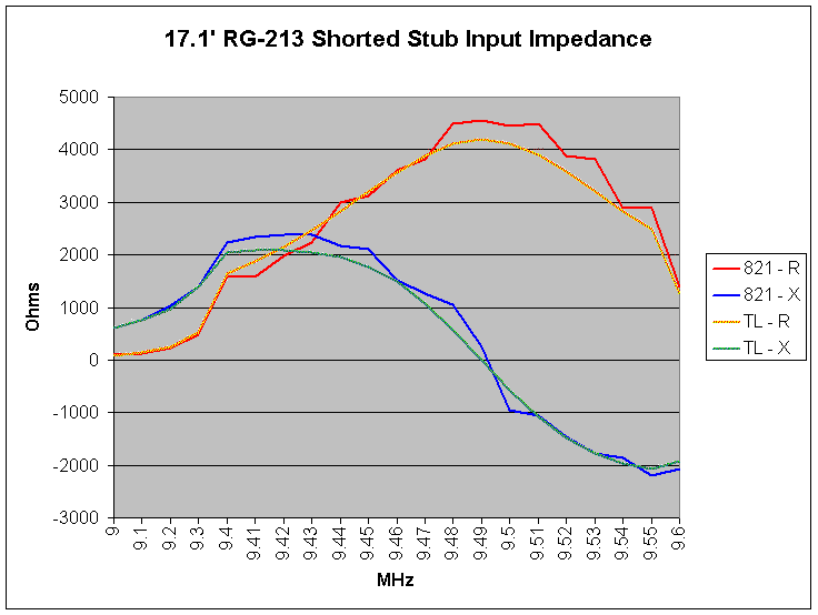
If my original measurements were correct, the frequency where the stub should be a 1/4 wavelength is 9.45 MHz. I decided to create a shorted stub, which should result in a high impedance at the 1/4 wavelength frequency. In theory, when we cross over that 1/4 wavelength point, the reactance should abruptly change from infinite inductive (+) reactance to infinite capacitive (-) reactance. I've always had trouble with this concept, since it seems so strange. I guess it's no stranger than the shape of the tangent function curve. By taking a number of readings around the 1/4 wavelength point, we can see the transition. This transition should also reveal the frequency where the stub is truly 1/4 wavelength.
I took my first measurement at 9.0 MHz, and made measurements in steps of 100 KHz until I got to 9.4 MHz. I then made measurements every 10 KHz through 9.55 MHz, which should surround the 1/4 wavelength boundary. Here are the measurements, along with the computed results from TLDetails.
| 17.1' of RG-213 Shorted Stub near 9.45 MHz | ||||
| GR 821-A Measurements | TLDetails Calculations | |||
| Frequency | Z | Q | Z | Q |
| 9.00 MHz | 97.08 + j 613.57 | 6.3 | 91.09 + j 601.43 | 6.6 |
| 9.10 MHz | 124.11 + j 766.25 | 6.2 | 141.16 + j 746.90 | 5.3 |
| 9.20 MHz | 219.56 + j 1028.40 | 4.7 | 247.09 + j 978.53 | 4.0 |
| 9.30 MHz | 475.31 + j 1400.62 | 2.9 | 530.90 + j 1385.97 | 2.6 |
| 9.40 MHz | 1597.09 + j 2238.77 | 1.4 | 1638.35 + j 2038.12 | 1.2 |
| 9.41 MHz | 1573.09 + j 2348.77 | 1.5 | 1877.53 + j 2077.43 | 1.1 |
| 9.42 MHz | 1989.14 + j 2386.73 | 1.2 | 2155.49 + j 2088.17 | 1.0 |
| 9.43 MHz | 2240.49 + j 2376.74 | 1.1 | 2473.19 + j 2055.02 | 0.8 |
| 9.44 MHz | 2989.92 + j 2169.20 | 0.7 | 2826.09 + j 1958.26 | 0.7 |
| 9.45 MHz | 3121.63 + j 2114.53 | 0.7 | 3200.30 + j 1775.43 | 0.6 |
| 9.46 MHz | 3599.40 + j 1515.16 | 0.4 | 3568.51 + j 1486.19 | 0.4 |
| 9.47 MHz | 3816.03 + j 1253.61 | 0.3 | 3889.04 + j 1081.27 | 0.3 |
| 9.48 MHz | 4494.94 + j 1062.04 | 0.2 | 4111.89 + j 573.36 | 0.1 |
| 9.49 MHz | 4567.13 + j 260.75 | 0.1 | 4193.98 + j 2.97 | 0.0 |
| 9.50 MHz | 4459.55 - j 958.28 | 0.2 | 4117.51 - j 568.89 | 0.1 |
| 9.51 MHz | 4499.10 - j 1068.13 | 0.2 | 3898.69 - j 1080.62 | 0.3 |
| 9.52 MHz | 3883.99 - j 1450.64 | 0.4 | 3579.81 - j 1490.37 | 0.4 |
| 9.53 MHz | 3823.26 - j 1781.40 | 0.5 | 3211.06 - j 1784.11 | 0.6 |
| 9.54 MHz | 2879.85 - j 1849.87 | 0.6 | 2834.90 - j 1970.35 | 0.7 |
| 9.55 MHz | 2898.85 - j 2204.52 | 0.8 | 2479.38 - j 2069.26 | 0.8 |
| 9.60 MHz | 1381.22 - j 2081.72 | 1.5 | 1256.98 - j 1928.58 | 1.5 |
Since we have a zero Ohm short at the output of the stub, we expect infinite Ohms at the input. With real lines, as opposed to ideal lossless lines, infinite Ohms means several thousand Ohms. The peaks in both resistance and reactance are visible in the data.
All of the Q values are very low. The resistance values are very high. The lesson here is that you can have a lot of resistance when using a stub. This is not a bad thing, and it's because the transmission line is really a transformer, not an inductor or capacitor. Let's say that you needed 1400 Ohms of inductive reactance at 9.30 MHz, and decided to build it with a 17.1 foot length of RG-213. You will indeed obtain that reactance, but the series resistance will be 475.31 Ohms. This value is clearly too large to ignore. If you are determined to use a stub to achieve a certain reactance, and you need a low resistance, you should explore the open and shorted versions, and in different cable types, and different lengths, to see if there is some combination that has an acceptable resistance. You could also place an actual inductor or capacitor at the far end of the stub, and use the transformed value at the input side. This would be a way to stretch more values from a smaller number of components by fronting them with coaxial transformers. This is what the professor did on Gilligan's Island to keep that old radio working.
I then used Excel to create a graph of the real and reactive components for both the measured and computed data..
|
|
| Comparison Between GR 821-A Bridge and TLDetails (Resistance and Reactance) |
I was quite pleased with the agreement between these two sources. TLDetails is working from nominal loss characteristics for RG-213 cable. If we were to measure and characterize the cable that I actually hooked to the bridge, we would no doubt have even more agreement.
The exact frequency where the cable is 90 electrical degrees is where the reactance changes sign, from positive to negative. TLDetails marks this as 9.49 MHz, and my measurements are closer to 9.495 MHz, a difference of 5 KHz. Before I made these measurements, however, I was calling the 90 degree frequency 9.45 MHz. This means that the 180 degree frequency is closer to 18.99 MHz, as opposed to my previously computed value of 18.9 MHz. I was off by 90 KHz at 19 MHz, which is 1 part in 190 or approximately 1/2 percent. While this is a low number, I really should go back to my first antenna analyzer page and recompute the expected impedance values, since they were all based upon knowing the frequency where the cable was 1/2 wavelength long. This small difference might change the agreement between the computed data and the measured data from the analyzers.
Armed with a sense that the results of TLDetails were reasonably close to the real transmission line, I computed the Q of the stubs in question.
The Sloper Array description is very terse. With respect to the transmission line stubs, it reads: Each dipole is cut to λ/2 and fed at the center with 50 Ohm coax. The length of each feed line is 36 feet. All of the feed lines go to a common point on the support (tower) where switching takes place. The line length of 36 feet is just over 3λ/8, which provides a useful quality. At 7 MHz, the coax looks inductive to the antenna when the end at the switching box is open circuited.
About all we can get out of this is that we have a 50 Ohm transmission line that is 36 feet long, which should be a little longer than 3/8 wavelength electrically. As mentioned before, an open stub provides capacitive (negative) reactance when it is zero to 1/4 wavelength long. From 1/4 to 1/2 wavelength, an open stub provides inductive (positive) reactance. Since longer lines imply increased loss, we might ask if it would be better to use a line which is under 1/4 wavelength long, and shorted, as an alternative mechanism to provide inductive reactance. There are two good reasons for the specified length. First, when using relays at the switching box, it's easier (less parts) in this design to generate an open as opposed to shorted circuit. More important, however, is the requirement that the physical transmission line must make it back to the center switching box. We know that a 40 meter dipole is approximately 66 feet long, or 33 feet to the center from an end. The end is claimed to be approximately 5 feet from the top. So, the distance from the top of the dipole support rope to the dipole center is near 40 feet. The dipole should make a 30 degree angle away from the tower. The sine of 30 degrees is 0.5, meaning that the projection of half of the dipole in the horizontal plane is 20 feet. The coax cannot be stretched so tightly that it will be horizontal. It will naturally droop. This adds to the length of the cable. If 36 feet is approximately 3/8 wavelength, then 1/4 wavelength will be around 24 feet. So, if we wanted to use a shorted stub under 1/4 wavelength electrically, the stub can never be longer than 24 feet, since that is 1/4 wavelength. It may be much shorter than 24 feet, depending upon the reactance we need. Given the natural droop in the cable, we cannot possibly be 24 feet or less in length. So, we have to move to the region between 1/4 and 1/2 wavelength, and if we want an inductive stub, it will have an open circuit at the far end.
Since the actual coax type was not specified, I started with the assumption that any old garden variety cable could work. The most generic cable to me is RG-8. I ran TLDetails, specifying an RG-8 cable, 36 feet long, at 7.15 MHz. Here are the results:
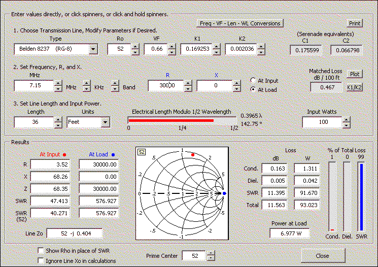 |
| TLDetails Results for the Sloper Array Stub |
We see that the velocity factor (VF) of this cable is 0.66, and that the electrical length is 0.3965 wavelength, which indeed is a little longer than 0.375 wavelength (3/8 wavelength). I simulated an open circuit with a load resistance of 30000 Ohms. At the input to the cable, the impedance is 3.52 + j 68.26 Ohms. Since the reactance sign is positive, it is an inductor. The Q of that inductor is 68.26 / 3.52 = 19.4. As inductors go, this is a rather low Q value.
This is equivalent to a perfect inductor with a reactance of 68.26 Ohms in series with a 3.52 Ohm resistor. The question becomes, how detrimental to the performance of the array is the additional 3.52 Ohm resistor at the center of the dipole? This will depend upon the radiation resistance of the dipole, since the loss resistance is in series with the radiation resistance. A sloping dipole at resonance has a resistance near 70 Ohms, but the mutual coupling to the other dipoles will lower that resistance, perhaps to the vicinity of 50 Ohms. The reduction in efficiency (loss) is approximately 7 percent, which is small - all things considered.
What if the transmission line was RG-58, which has more loss? According to TLDetails, the resistance increases to 6.96 Ohms, and the Q drops to 9.4. The miniature RG-174 coax has a loss resistance of 14.19 Ohms, and a Q of 4.5. While these Q values are very low, what really matters is the impact of the resistance at the feed point. In addition to the actual loss in power, the impact on the antenna pattern should be considered. This can be evaluated through a modeling program. Simply add the estimated resistance to the center of each parasitic dipole. This assumes that the modeling program is not performing the same computation as TLDetails, and adding the resistance in itself. Check with your modeling program, but the modeling programs I have seen use a lossless transmission line model which should not admit to the resistance of the stub - only the reactance. These are the little details that can cause a difference between a modeled antenna and a real antenna.
In the case of this design, the impact of the stub resistance appears to me to be small and not a major reduction in performance. If one picks a higher loss transmission line, however, the efficiency and pattern will degrade.
By the way, according to TLDetails, the length of a shorted stub less than 1/4 wavelength with the same inductive reactance as an open stub between 1/4 and 1/2 wavelength is a little more than 13 feet. Clearly 13 feet is too short to reach from the sloping dipole center to the switching box. There is no choice but to move out to the 36 foot length and switch from a shorted stub to an open stub.
On another page I described my 2-element 40 meter delta loop array using a parasitic stub to turn a loop into a reflector. The particulars of the stub were determined through antenna modeling. With this array I actually measured the current in the loops, and found that I could not achieve the amount of current in the parasitic loop which was suggested by the model. I measured approximately 80 percent of the expected current. Of course this difference degraded the response pattern. Could loss in the stub be the explanation for this problem?
My web page reports that the final stub length was approximately 33 feet. All of the cables I used are back in a cabinet, so I could recreate that length. I used my General Radio 916A impedance bridge to measure the stub impedance. In addition, I used TLDetails to compute the expected input impedance. Here are the results:
| Delta Loop Stub Impedance
and Q at 7.15 MHz (33' of RG-11U (VF = 0.78)) |
||
| Data | Impedance (Ohms) | Q |
| Measured on General Radio 916A | 1.56 + j 32.87 | 21.1 |
| Computed by TLDetails (RG-11U) | 1.41 + j 28.35 | 20.1 |
| Computed by TLDetails (RG-59) | 3.27 + j 28.29 | 8.7 |
The RG-59 computations show the impact of using a higher loss cable.
My cable measured a resistance of 1.56 Ohms, which was only 0.15 Ohms away from the computed value. Although a Q of 21 is low by comparison to lumped inductors, the resistance is low because the reactance needed is low. The radiation resistance of a loop, even with the coupling of a second loop, is probably around 70 to 100 Ohms. The 1.56 Ohm resistance which the stub adds to the feedpoint will add a very small amount of loss.
In the end, while there is stub loss which I was not taking into account, the amount of loss in and of itself does not appear to be large enough to account for all of the current reduction in the parasitic loop. I still suspect the impact of ground, and ground loss. The only solution for that problem is to get the antenna higher in the air, or, install a radial system under the array.
Coaxial cable stubs can present both resistance and reactance. It's easy to estimate (via calculation) the expected impedance of the stub, and then ask if the resistance is going to be a problem. In the examples I looked at, the Q of the equivalent inductor or capacitor was relatively low, especially compared to discrete components. In many cases, this will not be a problem in and of itself, and the stub will be a fine solution. With the Sloper Array and the delta loops, the use of a transmission line is essential since it functions both as transmission line and stub. It's this dual use which makes the whole thing clever.
If you are going to use a program like TLDetails, check to make sure that the cable modeled in it's computations matches the cable you are actually using. My RG-11 cable in the phased delta loop array had a velocity factor of 0.78. While TLDetails had two different RG-11 models, neither one had that velocity factor. I had to change the cable model so that it agreed with my actual cable. Be sure to check the impedance, the velocity factor, and the loss constants.
My Excel spreadsheet, StubQ.xls, can be downloaded by clicking on this link.
Back to my Experimentation Page