 |
| First Impedance Measurement |
Models and Measurements
Greg Ordy
It might come as a surprise, but I didn't even look at any models until the vertical was largely erected and complete. My goal was to get as much vertical metal in the air as I could, and then figure out what I could do to get it matched to 50 Ohms, with the highest gain and widest bandwidth. On the construction page, I left off with a 90 foot tall vertical that I called the Wet Noodle 90. My first impedance measurement and models were of this antenna. I was interested in the size of the base loading inductor necessary to resonate the antenna on 160 meters. So long as the inductor was relatively small, I would seriously consider using base loading for the first winter season.
This page looks at those results, and what I did based upon them. To chart out the general course before we get started, I found that the required inductor was larger than I wanted to use, especially after examining my previous large 160 meter loading coil. I was also disappointed in the bandwidth as suggested by a NEC model. This led me to add 3 top loading wires that doubled as guy wires and were attached to the very top of the antenna. This resulted in a smaller base loading coil, and a higher base resistance at resonance. This improved the bandwidth because the impedance step up was smaller. The antenna was also more stable in the wind, which is helpful when it's called a wet noodle.
The first measurement of complex impedance, resistance and reactance, produced the following graph. Please note that it's a sweep from 1 to 4 MHz in 5 KHz steps.
|
|
| First Impedance Measurement |
The blue data is resistance, and the pink is reactance. A couple of items are noteworthy. The red arrow points at some blips on the resistance (R) and reactance (X) data. These represent energy from AM broadcast stations. In particular, WTAM, 1100 KHz, is a 50,000 watt clear channel station not too many miles away from me. Although the VNA detector has a very narrow bandwidth, if you put the detector right on the frequency of a signal, it will detect the energy. The blue arrow points at a frequency region where the data has a few bumps and deviations from smooth curves. These are due to my 80 meter array that is less than one wavelength away from the 160 meter vertical. Coupling to those antennas shows up when measuring this 160 meter vertical.
What we care about is the data at the green arrow, which is the impedance in the 160 meter band. At 1.830 MHz, the impedance is 9.4 - j 166.3 Ohms. Perhaps the simplest way to match back to 50 Ohms is with an L network. I fired up the ON4UN Lowband DXing software, and used the L network module to provide solutions. In some cases, it's good to double check the results of that suite of programs. After entering my data, including 1.83 MHz, I had the following results:
 |
| First Matching Solution (Wet Noodle 90) |
I highlighted the first solution, which is also one that is correct, has reasonable values to construct or acquire, and is the one that is commonly used for shortened verticals. The L network consists of two inductors, one in series and one in shunt. As always, the shunt component is across the higher impedance side. Perhaps you thought that an L network needed to have an inductor and a capacitor. That's not true, it depends upon the impedance values. My first reaction was that I was hoping for a smaller inductor in the series arm. Although 12.76 uH is nothing like that 70 uH monster I just took down from the old vertical, it's still an indicator mocking me that my antenna is again too short. Ok, fine, but we can still press on.
The next step was to create a model of the antenna and the matching network so that we can evaluate the gain and bandwidth.
For some reason, at this point, I decided to do something that I think about doing, but never really have done to this degree before. I decided to see if I could get a model to track my measured resistance and reactance as closely as possible. Since my actual vertical is a triangular lattice tower with many tapers, ending up in tubing that telescopes, I was not going to model all of that. I was interested in finding a length of aluminum with a certain diameter over the MININEC ground model that matched what I measured. After a little but of trial and error, I ended up with this comparison.
 |
| Modeled and Measurement Comparison |
Hopefully it's clear that under 2.8 MHz the model and the measurement track very closely. Above 2.8, I believe that the measurement is under the influence of the nearby 80/40 meter vertical array. If we get very specific about comparing the data in the 160 meter band, we see this:
 |
| Modeled and Measurement Comparison |
At 1.830 MHz, the resistance error is around 0.2 Ohms, and reactance is around 1 Ohm. I thought this was very good agreement, and I especially like that it was tracking together, as opposed to just crossing at some impedance value. Ok, so, we know what the real antenna looks like, but what sort of model produced nearly the same results? The NEC-2 model, captured in the EZNEC+ program, was of an aluminum wire that is 78.5 feet tall and 14 inches in diameter.
I hope that's not shocking or alarming. With NEC-2 in particular, the modeling of stepped/tapered diameters is known to be not accurate. This has led to the stepped diameter correction that many NEC wrappers, such as EZNEC, use. This is a correction to a model, before simulation, that converts a model consisting of multiple diameters into a model of a single diameter and an equivalent length. Now there are many issues surrounding this correction, and we have other fish to fry on this page. But, when I knew that my actual antenna was 50 feet of triangular tower that tapers from 22 to 11 inches, and that the upper 40 feet are telescoping tubing from around 2 inches down to 1 inch, the odds are good that an electrical equivalent will be less that 90 feet tall, and fatter than 1 inch and thinner than 22 inches. I fooled around until I found 78.5 feet long and 14 inches in diameter as being very close. I guess you could call this a manual stepped diameter correction.
Because of the close tracking of impedance, I'm going to use the updated dimensions as a proxy for the actual antenna. Since I'm looking at issues of matching and bandwidth, impedance is probably more important that some other parameter such as gain. I should also mention that I did not add any base resistance to the model to achieve tracking. With the MININEC ground model, ground system loss is usually modeled as added series resistance at the base. So, it is probably also reasonable to say that my ground loss is low, since I was able to get an impedance match with an antenna with zero added loss. If you try to match your measurements to models, and you can't quite make it work, be sure to think about what ground loss you might have in your system, and if it's represented in the model.
We now have a model of the antenna and values for an L matching network that promises to transform the base impedance to 50 Ohms. the next step is to add the matching network into the model and look at the performance. We could have a big discussion about how to model an L network in EZNEC. Historically, you would construct an L network out of NEC loads. On one hand, this is a little complicated, since you have to get the series and parallel configurations correct and understand a bit more about how NEC works. The good news about using two interconnected loads to model an L network is that you can get complete voltage and current information for the parts. This can be very important, especially if you are trying to figure out power levels and component ratings. More recent versions of EZNEC include a specific L network primitive, which is much easier to use. If there is a problem with that approach, it is that, to the best of my knowledge, it's not possible to get information on the voltages across and current through the parts. This is because the L network primitive maps to the NEC-2 network primitive, as opposed to the NEC-2 load. So, the approach choice may depend upon what information you are looking for. In this case, I'm going to use good old fashioned loads, since I can get as much information as exists for them.
I added the two loads to the model. I should also mention that these are ideal loads, that is, lossless. Neither inductor has any resistance, only reactance. This is unreasonable, especially as the inductance rises, but, it's a common starting point. I ran an EZNEC sweep, and then used the LBDXView program to plot the SWR. Here is the result, sweeping from 1 to 4 MHz.
 |
| SWR of Modeled Antenna and L Matching Network |
Whoa, from that perspective, this is very narrow banded. But, if we restrict the frequency to the useful range of 1.8 to 1.9 MHz, we see the following.
 |
| SWR of Modeled Antenna and L Matching Network (160 m) |
Now I should have hit an SWR minimum of 1.00, not 1.08. There is a little bit of slop and rounding errors going on. We did, however, hit the target frequency. So, is this good enough? I guess that's up to each of us to decide. In this case, however, the SWR bandwidth under 2.0 is slightly less than 50 KHz. I was hoping for a little more. Depending upon what we are interested in, we could run a lot of variations at this point. One that I will run is to add some loss resistance to the inductors. As an example, let's add 1 Ohm of resistance to the 12.76 uH loading inductor, which represents a rather poor Q of 150 (Q = X / R). Let's also add 0.1 Ohms of resistance to the smaller 2.09 uH matching inductor. This is a more respectable Q of 240. The EZNEC loads window now looks like:
 |
| EZNEC Load Window for L Network With Loss |
I swept the 160 meter band again, and graphed the two SWR values (with and without loss) and also the power (in watts) consumed in the two loads. The input power has been set to 1500 watts. The result is:
 |
| SWR and Power Loss of Modeled Antenna and L Matching Network (160 m) |
We can see that adding in some loss made the bandwidth slightly wider (green trace), which is often what loss does - makes an antenna look better from an SWR point of view. That's why, although SWR and matching is important, it should not be used as the sole indicator of performance. After all, a dummy load has a really excellent SWR. The power consumed by the larger loading inductor is around 140 watts (out of 1500), and the power in the smaller matching inductor is a much lower 14 watts. If you are building these inductors, you should be sure that your components can handle the suggested levels, with perhaps a safety margin. We probably also care about the reduction in antenna gain due to the addition of loss. That can be plotted against the SWR, and it looks like:
 |
| SWR and Gain Loss of Modeled Antenna and L Matching Network (160 m) |
The drop in gain appears to be around 0.4 dB. If you are going to be closely comparing gain values to make choices, be sure that you factor in loss when possible. If not, you could arrive at incorrect conclusions. The Q of large inductors, especially in series loading locations, matters. They can have large voltages across them, large currents through them, and dissipate significant power. This means that they can influence the antenna gain. I'll compare the this inductor voltage and current to the final inductor later on this page. For now, let me say that the voltage across this inductor is around 1750 volts, and the current through it is around 11.5 amps. Large loading coils, common on 160 meters, can develop a hefty voltage across them. This could raise a safety concern if the inductor is at the base of the antenna, and demand the use of vacuum relays if you want to be switching the ends of the coil.
In my case, another factor on my mind was watching the Wet Noodle 90 sway in the wind. I was slowly concluding that having a third set of guy lines going to the very top would be helpful. I decided to combine that guying with some top loading. In other words, the first segment of these new top guy lines would be wire. They would terminate at an insulator, and then finish their trip to the ground on 3/32" UV Dacron rope. I did go through some models to see what that top loading brought to the table. Since the lines are folding back towards the ground like an umbrella, there are trade offs. As you make the lines longer, the loading increases, which is good. On the other hand, because the lines are running downward while the antenna is running upward, there is some current cancellation, and loss of gain. So, I want some top loading, but not too much. After looking at several alternatives, I picked 20 feet, mainly because it was a round number in a range that seemed helpful.
Here is an updated diagram of the Wet Noodle 90, now with 3 additional loading/guying lines. I should probably drop the wet noodle name, since the antenna is now very stable in the wind.
 |
| Top Loading Wires |
Here's what the 3 levels of guy lines look like from the ground.
 |
| Real Top Loading Wires |
Generally speaking performance and bandwidth will increase the higher up a vertical you locate a loading device. The idea is to have the longest section of conductor under the loading device since the loading device will change and reduce the current profile on the antenna. Since alternating current leads to radiation, more current is good. Loading inductors on standing wave antennas drop the current to the top side of the inductor, and, therefore, it's desirable to get them as high as possible. This leads to the sense that top loading is preferred to center loading, and center loading is preferred to base loading. Both L.B. Cebik, W4RNL (SK) and John, ON4UN, have written on this topic.
After adding the wires, I again measured the impedance at the base. The captured data was:
 |
| Real Top Loading Wires |
The impedance at 1.830 MHz, with the top loading wires, is 14.65 - j 108.70 Ohms. Without the wires, the impedance (first graph) was 9.4 - j 166.3 Ohms. The reactance to tune out the resonance has dropped from 166 to 108 Ohms. That drops the required inductance. Perhaps more important, the resistance rises from 9.4 to 14.65 Ohms. That's very good news because the bandwidth of an L network is related to the size of the impedance transformation. 14.65 to 50 Ohms is a factor of 3.4, whereas 9.4 to 50 Ohms is 5.3. This means that the system bandwidth will increase, due to the smaller impedance step in the matching network.
At some point it's necessary to determine if we want or need to have a second SWR dip provided by the control box. I had already designed the PCB to provide a second dip, so, I decided to use it. That means that the first dip, without the added series coil, needs to be higher in frequency since the second dip will be lower in frequency. I picked 1.850 MHz, where the impedance was 15.09 - j 104.74 Ohms. Putting this target into the ON4UN L network software provided a solution with a series inductor of 7.04 uH. and a shunt inductor of 2.93 uH. The drop from 12.76 uH to 7.04 uH is almost a two to one drop, so that's taking a big bite out of the inductor.
From looking at the table of measured reactance, I determined that an additional inductor of 0.6 uH would shift me down from the SSB portion of 160 meters to the low end of the CW segment.
I now had all of the inductor values I needed. The series loading inductor is 7.04 uH. The matching shunt inductor is 2.83 uH. The shift down second SWR dip inductor is 0.6 uH. These are the values recorded on the schematic on the control box page.
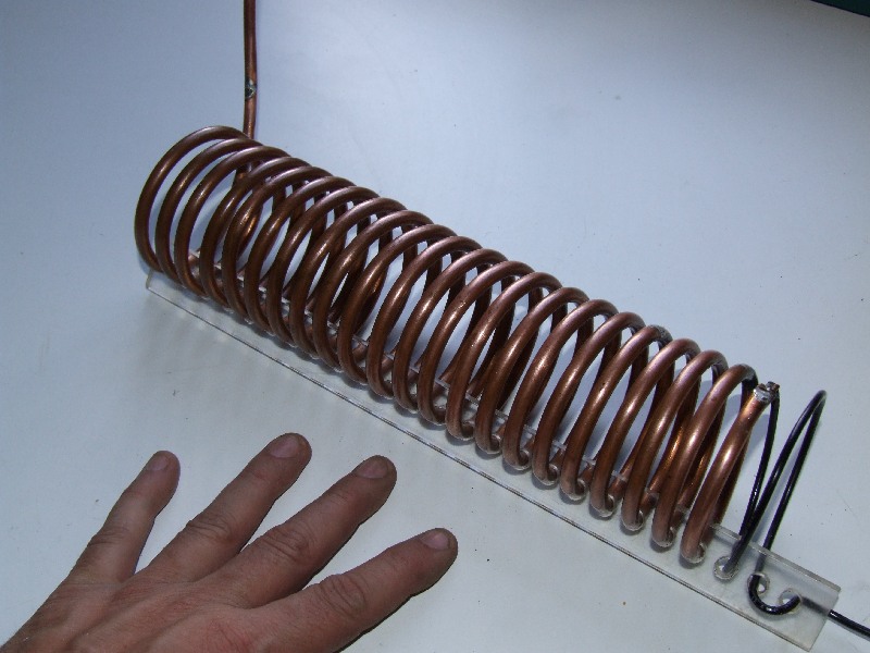
The 0.6 uH coil is three turns of #12 insulated wire wound on a form around 2 inches in diameter. There is a lot of space between the turns. The 2.83 uH matching inductor is wound on a T225A-2 powered iron core. This is a 2.25" O.D. double height mix 2 (red) toroid. The 7.04 uH loading inductor was a bigger challenge. First, unlike the other two inductors that were inside the control box, this inductor goes from the control box to the actual tower. That means that is needs to span around a foot of distance. It has a mechanical and electrical function. While I might be able to wind it on a toroid, that level of compactness is simply not needed. As I was playing around with alternatives, I remembered that I had some inductors that I had never used with my original 160 meter vertical. Unlike the big monster 70 uH coil, these were much smaller coils, although constructed from the same copper tubing. In fact, these were my original center loading coils, wound around a dozen years ago, but I abandoned them in favor of the big monster. Could they be reused here?
I retrieved the longest from a box, and checked its inductance. I had almost 2 feet of coil, so I knew I had far more than enough. I made some measurements that suggested where I should cut the coil, and I did. Well, as often happens in life, the light bulb in my brain went off just a little bit late. I further remembered that I should also have a few of the plastic spreader arms that I used to wind the original coil. It struck me that if I could thread this smaller coil through a single spreader arm that I would have a great coil support backbone. I was indeed able to thread the coil through the arm, and it's exactly what I wanted for mechanical reasons. Unfortunately, the arm caused the turns spacing to increase enough that my coil was now short on inductance. The 7.04 uH dropped to 6.85 uH. I compensated with an extra turn or so made from solid #12 insulated wire that was going to run to the ceramic feed through on the control box anyway. Here's a picture of the final loading inductor, along with my hand for a sense of scale.
 |
| Loading Coil and Human |
So, it's a little strange, but quite functional, and the plastic bar keeps the coil rigid and supported. I bent a turn straight at one end of the coil, and this is clamped to the tower leg with two hose clamps.
Here is the loading coil, mounted on the tower and the control box.
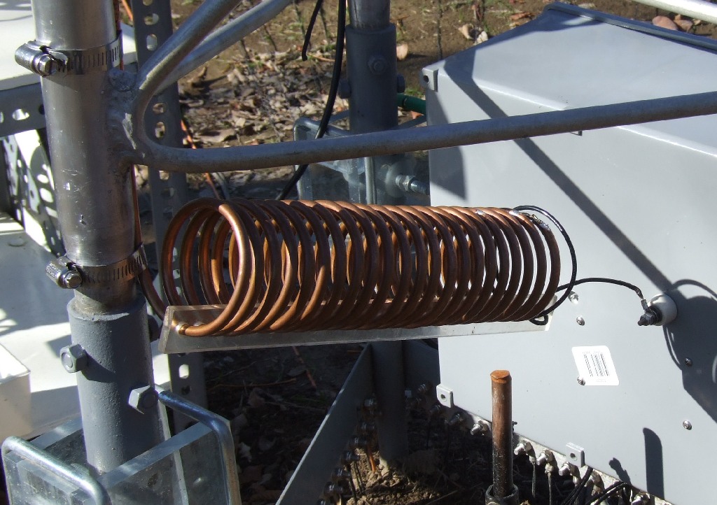 |
| Mounted Loading Coil |
After all of the foreplay, it all comes down to the curves for the two SWR dip choices in the control box. The SWR curves for the two control settings are:
 |
| Mounted Loading Coil |
I ended up with dips near 1.820 MHz and 1.850. The SWR is under 1.5 from 1.800 to 1.870, which is most of the band that I would use. Compared to my previous vertical, this is a big increase in bandwidth. For a single dip, the 2 to 1 SWR bandwidth appears to be 90 KHz. The initial wet noodle had a 2 to 1 bandwidth of around 50 KHz. So, the top loading did it's job, and the bandwidth increased. That really was my main goal, more bandwidth.
I did update the EZNEC model with the top loading wires and the new inductor values. I again used the 78.5 foot tall antenna as the starting point, and modeled the top loading with #14 wires. This meant that the loading wires were closer to the ground since the equivalent antenna was 78.5 not 90 feet tall. So, you figure that this is going to introduce some error in the response. I added resistance to the new inductors to match the Q values of the first models. Given that, let's compare the two versions, with and without top loading wires.
Let's start with voltage across and current through the two loading inductors.
 |
| Loading Coil Voltage and Current Comparison |
The voltage across the loading coil dropped from around 1750 volts to a little less than 800 volts. This could be important if relay contacts were involved on both sides. The current drops from around 12 to around 10 amps. The power dissipated in the loading coil drops from around 140 to around 50 watts.
Finally, let's compare the gain:
 |
| Antenna Gain Comparison |
The gain difference due to top loading is very little, so of this all comes down to bandwidth. A full size vertical, without any lossy loading devices, has around an additional 0.5 dB gain. Although we saved around 100 watts with the smaller loading coil, that potential gain was offset by the loading wires folding back towards ground.
The last step in this antenna project was to add a warning sign to the base. I was pretty lucky in the timing. Less than a week after adding the sign, we had our first snow.
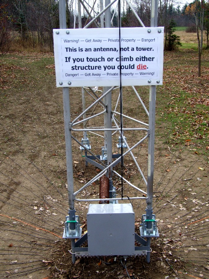 |
| Tower Warning Sign |
Back to the 2010 W8WWV Vertical Page
Back to my Experimentation Page