 |
| 4-Square Element Currents |
Greg Ordy
My experience with phased arrays suggests that unless you measure the actual currents in the elements you can never be confident that you have constructed the desired array, especially if mutual coupling between elements is present. This is not to suggest that your work up to the current measurements can be sloppy, and you can then tweak the system into perfection. Far from it. My experimentation tells me that it is essential to be very precise and careful in all steps that lead to the design and implementation of the system, but no matter how careful you are, tweaking of the phasing network will still be required.
One of the tools which can be used to analyze the element currents is the oscilloscope (scope). This page describes my approach to using the scope to make current measurements.
Why should we want to be so precise about the phasing? Here are a few thoughts to keep in mind.
Even if we achieve our desired phasing, those conditions will exist at only one frequency. As you change the frequency by even a few KHz, the currents will begin to change.
Array gain and the RDF metric usually hold up well against phasing errors. In other words, a so-called casual phasing network, which has substantial error, will reduce the gain and the RDF by relatively small amounts.
Sharp nulls, on the other hand, are very sensitive to phasing errors. You will never achieve the deep 20+ dB nulls seen on antenna response patterns unless you have very specific current relationships.
If you are building a Gehrke-style phasing network, the array feedpoint impedance, and, therefore, the SWR on the transmission line back to the radio, are directly tied to phasing errors. Phasing is combined with input impedance matching. If the phasing is wrong, your SWR will not be 1.0 at the target frequency. Note, having a 1.0 SWR is not a guarantee that the phasing is correct.
The sharp nulls in the antenna response are usually desirable for reception, not transmission.
The particulars of your application may help determine the degree of phasing accuracy needed. For example, a station might decide to use a 4-Square array exclusively for transmission, and do all reception on a set of Beverage antennas. In this case, the phasing accuracy really doesn't matter. On the other hand, precise phasing control might be desirable to neutralize persistent noise from a particular direction on reception.
To be honest about it, my reason for trying to measure the phasing and then optimize the network is because it's there. If you are building a phased array, you have already designed and constructed at least 2 elements, built a phasing network, and built a direction switching network. Why would you do all of that work, and not be sure that you attained the desired result? It's the final major step of the job. It's also a certain amount of fun, although it can be very frustrating, especially when you are trying to adjust the network. I have found that working with the scope at least provides a complete set of current magnitude and phase information.
Although the information on this page can apply to a wide range of phased arrays, my experience and the examples come from arrays of vertical elements used on the 160, 80, and 40 meter amateur bands.
I believe that the performance truth about an antenna (especially the response pattern) is largely contained in the physical dimensions and spatial relationships of the elements as well as the element current magnitude and phase. I have often times taken measured current data and used it as the sources in my antenna models (with EZNEC). The antenna modeling software then shows me the response pattern for what I have actually built. This is especially useful in investigating the antenna performance as you tune away from the target frequency (and performance begins to degrade).
Much of my phased array work begins with these references.
Vertical Phase Arrays, by Forrest Gehrke, K2BT. This six-part series appeared in Ham Radio magazine between May of 1983 and May of 1984. It is probably the most quoted source of phased array information (for amateurs) - covering all aspects of their design and construction. Unless you have access to copies of the magazines, the only other way that I know to obtain this information is to purchase the Ham Radio CD-ROM archives from the ARRL. As luck would have it, this series crosses two different products, so you have to purchase two sets to get all six articles.
Low-Band DXing, by John Devoldere, ON4UN. In the third edition, chapter 11 covers vertical phased arrays.
ARRL Antenna Book, by the ARRL. The Multielement Array chapter covers phased arrays.
The web pages of Tom Rauch, W8JI. Tom describes a type of phasing called crossfire phasing. This approach has the property that the phasing network is largely frequency independent. When coupled with broadband antennas, the result can be excellent performance across several amateur bands. Ideal for receiving antennas, this is only way I know of to get away from the problems associated with narrowband antennas (and narrowband feed systems).
Other references are contained on my Resources and Links page.
If you search the Internet, you can find several tutorials on general scope theory and operation. Most seem to be associated with college courses, and I hesitate to provide links since they seem to shift from semester to semester.
The scope is not the only part of the current measurement system. Since we want to measure current, the process begins with current probes. My current probes are described on another page. The current probe location is also important. In the case of vertical elements, the probe is usually located right at the bottom feedpoint. The current probe is inserted in series between the transmission line and the antenna.
The probe transforms the current going into (or out of!) the antenna into a voltage level. A shunt resistor which matches the impedance of the transmission line helps the line run flat, without an impedance transformation effect. When a transmission line is not terminated in its characteristic impedance, it acts as a transformer. In this application, that behavior is undesirable.
I use RG-8X 50-Ohm cable with my current probes. I have six, 48 foot long runs which have been cut for this purpose. I have six elements, so I need six current probes and six cables.
The transmission lines just mentioned transfer the signals at the current probes to a common point where the scope will sit, and actual measurements will take place. It is very critical that the probes and the transmission lines be symmetric, that is, all the same. What is important is the electrical length of the cables, not their physical lengths. The two different lengths are related by the cable velocity factor, which is not necessarily constant (especially between different batches and brands). What I do to check the equipment is to put two probes in series, so that they sense effectively the same signal. I then pick two of the cables and verify that the scope shows the same trace for each signal. I rotate through all pairs of probes and cables. This scheme provides some confidence that the probes followed by the transmissions lines all report the same voltage for the same current. I have dedicated those cables for this purpose, and have used them with several different antenna arrays.
The current probe itself will introduce small phase shifts in the elements. My probes consist of several inches of wire run through a ferrite core. This wire adds length to the antenna which will be removed when the probe is removed. At low frequencies, the error added is very small. Still, keep all wiring as short as possible. If I wanted to measure the currents in a 2 meter Yagi, I would have to develop a whole new approach with the required accuracy. Those few inches of wire which can be neglected at 80 meters would cause total chaos and confusion at 2 meters. One solution to this concern would be to simply leave the current probes in the system at all times. This could be part of a continuous monitoring system. In this case, be sure that you can handle the signal that comes off of the probes when you move to high power. Another alternative would be to replace the current probe with an equal length wire. I'm being very anal here, since the error introduced at the low frequencies is very small.
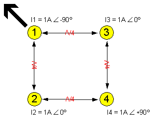
In some cases, it may not be necessary to measure all of the elements in an array. This is usually true when two (or more) elements should have identical currents. Assuming that identical elements are connected by electrically identical transmission lines, which are driven in parallel, and all other aspects of the array are symmetric, then one is strongly led to believe that the current in one element matches the current in the other(s). Consider the following example, the 4-Square antenna array.
|
|
| 4-Square Element Currents |
The array fires through a diagonal. Elements 2 and 3 have identical currents, 1 amp at 0 degrees. Each of those elements is also the same distance and orientation from the other three elements. If the phasing system feeds elements 2 and 3 through identical length cables, and then combines the cables in parallel at the network, the currents in those elements should be identical. The final constraint is that elements 2 and 3 should be identical, and have identical radial systems. In that case, it is not essential to measure all 4 elements. You can measure elements 1 and 4, and either 2 or 3. This would be helpful if you had a three channel scope, but not a four channel scope.
My own approach is to initially measure all elements, and confirm that the elements I believe are identical really are identical. Even if I'm not going to measure a certain element, I will still insert a current probe at the feedpoint, and connect the cable back to the scope position. This is my attempt to have the probes introduce the least error into the system, and if there is going to be error, it should be introduced equally to all elements.
The scope is the central focus of the current measurement. Fortunately, the demands on the scope are relatively few, and many inexpensive used scopes will work just fine.
The scope should have a bandwidth which is greater than the frequency of interest. If you are going to build a 40 meter network, the scope bandwidth should be some safety margin above 7 MHz. Common scope bandwidths such as 60 MHz should work for all HF bands.
The scope must have at least two channels, and ideally as many channels as you have network legs. I use the term leg as opposed to element (or antenna), since in some arrays several elements may be combined in parallel, creating a single leg. In the case of my array, I have 6 elements (vertical antennas), but only 3 legs because pairs of elements are combined in parallel. There would be nothing wrong with monitoring all 6 elements with a six channel scope, but those are hard to find. After verifying that the array is truly symmetric, I can measure the array with a three channel scope, one channel per leg. I have confidence that the three elements not measured will very closely match the three elements I am measuring.
I purchased a used five channel scope through eBay. In 2002 it cost $225 dollars (USD). I use three of the five channels in the Hex Array project. It is also necessary to have an adequate supply of BNC adapters and connectors. Most all scopes I have ever seen use BNC connectors. My current probe signals arrive at the scope on a PL-259 connector. I need an adapter to convert to BNC, then a BNC Tee which allows me to add a 50 Ohm termination at the scope input. I have accumulated a large box of BNC plumbing over the years, and it's needed to create various lash ups. This is especially true if I need to make up more than one of a certain configuration. These are good hamfest items. If I buy nothing else, I buy some BNC hardware.
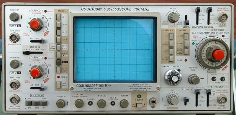
Here is a picture of the scope and some typical BNC connectors/adapters/plumbing. Please click on a picture for a larger view.
 |
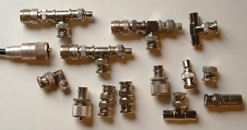 |
| Kikusui COS6100M Oscilloscope | Typical BNC Parts |
A few comments on scope channels. The most common number of channels is two. If you have two legs, then a two channel scope is perfect. If you have more than two legs, you may be tempted to try and use a two channel scope. While this can work, the problem is that some leg will be invisible when it is not connected to the scope. This will lead to the false sense that it is not changing as you adjust the phasing network. This is usually not true. So, you will need to swap channels frequently in order to have a complete picture of what's going on. If possible, get as many channels as you need, not just two.
It is also the case that most scopes will only have two channels with high sensitivity. Scope channel sensitivity is specified in the amount of voltage necessary to deflect the trace vertically by one division. The first two channels usually have very sensitive and adjustable front ends which can provide vertical sensitivity down to the microvolt level. This is not usually true for any channels beyond the first two. In the case of my scope, for example, channels 3, 4, and 5 have two fixed positions, either 0.1 volt per division, or, 1.0 volt per division.
In order to simplify reading the scope traces, it is desirable to operate all channels with the same sensitivity. As a result, when I use three channels, I set the sensitivity of each channel (A, B, and C) to 0.1 volts per division. A trace should also fill most of the vertical dimension of the screen, which might be 6 to 8 divisions. This means that the peak to peak voltage swing needed from the current probes is around 0.6 to 0.8 volts. This will impact the amount of drive power which must be inserted by the signal generator in order to make useful measurements. A later section talks about this in more detail. The practical impact is that when I need to use more than two channels, I can no longer use my MFJ antenna analyzer as a signal generator - it does not supply enough power. I have to switch to a more typical signal generator.
A final comment about scope channels. In order to allow the user to map arbitrary voltage levels to full scope divisions, the first two channels usually can be put into an uncalibrated mode where the sensitivity is continuously variable. Make sure that this feature is not turned on, and that all channels are set to the same sensitivity. If they are not all the same, and all calibrated, then the readings will be apples and oranges, difficult to compare. The calibration knobs are usually part of the rotary sensitivity switch, and can be easy to accidentally turn. I know, I've done it. If you have a concern about the channel calibration, swap inputs and verify that does not change the readings, other than to swap them.
The scope has a horizontal time base, which controls the rate at which the trace is drawn, from left to right. Unlike the channel sensitivity settings, which should always by operated in the calibrated mode, the horizontal time base in this application is always uncalibrated. This allows me to stretch or shrink the waveform so that a full 360 degree cycle exactly lines up with scope divisions. This is the basis of measuring phase, the mapping between divisions and trace peaks (or whatever reference point you select, zero crossings, for example).
The scope must be triggered by one of the channels. I usually pick the leg which I consider to be the reference leg. This leg usually has a relative phase of zero degrees. Triggering and the horizontal time base are synchronized so that each time the electron beam is drawn, it draws on top of the same signal from the previous trace. This provides a stable display. If the traces are unstable, and appear to be rolling across the screen, you need to adjust your triggering polarity and/or level.
The scope face is divided into a grid of divisions, which are further divided by ticks. A common configuration is 8 vertical divisions and 10 horizontal divisions. Ticks commonly divide the division into fifths. In other words, each tick is 0.2 division.
In recent years, the digital storage oscilloscope has become popular. It's a combination of the traditional analog scope, and the traditional logic analyzer. Like the logic analyzer it stores captured data in digital memory. Unlike the logic analyzer, where each point is a simple binary (on/off) value, each point is a number which represents the magnitude of the signal. This makes it possible to display signals such as a sine wave, which a logic analyzer can't process. Handling of this continuous analog input data requires channel processing like that found on a traditional scope. For this reason, the DSO usually has a small number of channels, as opposed to the logic analyzer, which might have 16, 32, or more channels.
Perhaps the best feature of the DSO is its ability to capture fast single events. The traditional scope is best for monitoring periodic signals, since it is constantly redrawing the screen as a function of the input (no internal storage). In this application, however, we do have constant sine waves, which are ideal input signals for the traditional analog scope.
DSOs tend to have relatively low bandwidths, unless they are very expensive. In my application, under 10 MHz, that is not a problem.
The DSO has been combined with the LCD to create small, lightweight, handheld scopes. The only drawbacks are their cost, and I have never seen one with more than two channels. But, they are very convenient. When I want to make phase measurements on my array with the setup described on this page, I literally fill up a wheelbarrow with heavy test equipment, and have to run about 300 feet of extension cord to provide AC power from the house to the antenna site. I won't do this when the weather is bad (mainly wet), and that can be at least half of the year where I live. One of the battery powered handheld DSOs would simplify outdoor measurements, and could be used all through the year. Check out popular manufacturers such as Fluke, or suppliers such as Jameco.
A variation on the DSO is a unit that captures data but then uses a computer for display and control. When combined with a laptop/notebook computer, the solution is almost as portable as the dedicated handheld scope. One unit that has caught my attention is made by Scope4pc. Having four input channels, it is ideal for most arrays.
Because DSOs store the waveform in memory, they can post process the data and characterize the signal. Many of the products can display magnitude and phase information as numbers, in addition to displaying the waveforms. That can simplify the analysis of the phase information (just read the numbers!).
My only concern about this approach is the latency between data capture and data display. The traditional scope continuously updates the waveform on the screen. Adjustments are immediately visible. With the DSO, a capture must be triggered then processed. While these units have a continuous trigger/update mode, I wonder if there is a delay between the actual signal and the waveform display on the screen? This is especially true in the case of the box that uses a PC for display and control. If the delay is too long, then the visual feedback while tweaking the network will be sluggish and awkward.
In order to measure current, we must drive the array with RF power at the design frequency, which will supply current for the elements. My favorite signal generator is the common antenna analyzer, such as the MFJ-269, or the AEA HF-CIA. These devices emit a low level signal as part of the impedance measurement process.
When using an antenna analyzer as a signal generator, it is possible to monitor the feedpoint impedance and SWR at the same time that the element phasing is measured. This is very helpful when using a Gehrke-style feed system. With that design approach, a properly adjusted network provides a 50 Ohm (resistive) feedpoint impedance while also providing the desired currents. So, you really need to measure input impedance as well as currents at the same time.
The antenna analyzer stops being effective when you need more power than it can provide. When you can no longer use an antenna analyzer, it's time to switch to a standard RF generator. I have an old but beautiful General Radio 1330 generator which I picked up from George, W5YR. Here is a picture of this classic device which uses vacuum tubes, and is built like a battleship. Please click on the picture for a larger view.
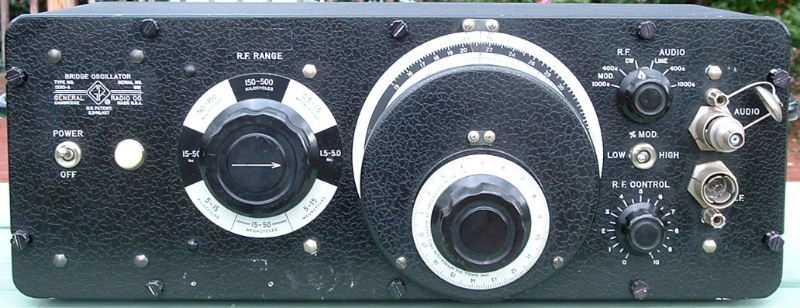 |
| General Radio 1330-A Bridge Oscillator |
This generator can provide a signal which appears to be 5 to 10 times stronger than the MFJ-269. When I use the 1330, I still use the MFJ-269, but this time as a digital frequency counter, which provides a simple and accurate readout. Dedicated signal generators usually have variable output levels, and that feature can be of great value in setting the height of the scope traces so that they largely fill the screen vertically.
There is nothing wrong with using an actual transmitter as a signal generator. It's hard to believe that it would ever be necessary to supply more than a few watts to an array under measurement. This means that the transmitter should have an adjustable RF output which can go as low as a few watts, and that the transmitter can tolerate being on for minutes at a time. In my case, I would use my ICOM IC-706MKIIG, which is physically small, and can throttled back to a few watts. To date, that has not been necessary.
When It's time to make phase measurements, I load up the wheelbarrow with the scope, the signal generator, the antenna analyzer, related cables and probes, the schematic, tools, the folding card table, and a chair. I cart the load out to the center of the array, where the control box is located. I also have to run an extension cord back to the house for 120 VAC power.
Here is a picture of the setup. Please click on the picture for a larger view.
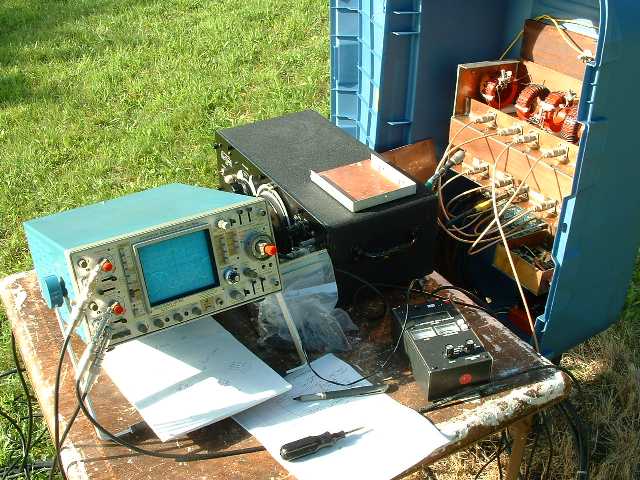 |
| Phase Measurement Field Setup |
I select the three legs which I want to monitor, and connect then to the A, B, and C channels of the scope. My phasing networks are located in the boxes in the plastic enclosure on the right. The trimmer capacitors are located between the red toroid inductors mounted vertically.
Just to make sure that the test configuration is clear, here's a little colorful abstract block diagram that shows that big picture that everybody is talking about.
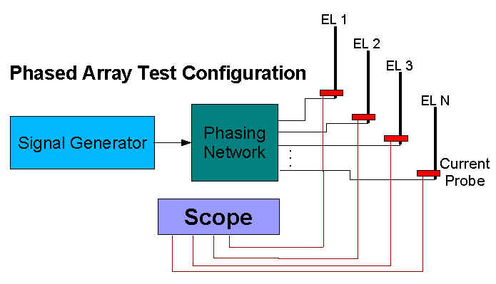 |
| Test Configuration Block Diagram |
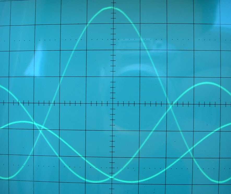
Finally, it's time to look at some scope traces. The following picture shows the phasing of my Hex Array on 40 meters. Yes, if you look closely you can see my reflection on the screen as I snap the picture with my digital camera.
 |
| 40 Meter Phasing |
Each trace (sine wave) represents one leg in the network. The peak to peak height of a trace indicates the current magnitude of the leg. The phase shift can be computed by picking some reference point on the trace, and then measuring the shift relative to one cycle of the reference trace. I pick the tops of the waves as the phase reference points.
The design had current magnitude ratios of 1 : 2 : 1. That, is the middle or center leg, which is also the Reference Leg, has twice as much current as the front and rear legs. The middle leg is assigned a relative phase of 0 degrees. The front leg (director) has a lagging phase of -120 degrees, and the rear leg (reflector) as a leading phase of +120 degrees.
I drop all of the traces to a common bottom division line. The traces are dropped by using the vertical offset control for each channel. Current magnitude is then the number of divisions and ticks above that line to a particular peak. I adjust the output of the RF generator to set the vertical height to be most of the screen, and to line up with division lines. NOTE: do not adjust the height of a trace by changing the channel vertical sensitivity, since that will throw off the relationship between the channels. Most array designs will specify current magnitude ratios using small integers, such as 1 : 1, or 1 : 2 : 1, or 1 : 3 : 3 : 1. What we have to work with now are scope divisions and ticks. I tend to count up the ticks, then divide all of the counts by the smallest tick count. This creates ratios where the smallest value is 1, and the other magnitude values will be greater than 1. See the 80 meter section below for an example.
I have decorated this picture with several numbers which match the following descriptions.
Marker 1 indicates the Reference Leg. This is the leg which should have twice as much current as the other two legs, and is assigned a relative phase shift of zero. I center it on the screen horizontally to indicate zero. The peak of this wave is centered over the vertical center line. The Reference Leg has a magnitude of 6 divisions, and the other two legs have a magnitude very close to 3 divisions. This reflects the desired 1 : 2 : 1 magnitude ratio.
Marker 2 is the lagging phase leg, the one targeted for -120 degrees relative to the reference. Since the traces are drawn from the left to the right, traces to the right lag traces to the left.
Marker 3 is the leading phase leg, the one targeted for +120 degrees relative to the reference.
Marker 4 shows how 180 degrees of the Reference Leg maps to 3 divisions on the screen. If 3 divisions equals 180 degrees, then each division equals 60 degrees, and each tick mark is 12 degrees. I adjust the horizontal time base in the uncalibrated mode until 180 degrees matches (spans) 3 divisions. The horizontal position must be adjusted at the same time to keep the peak of the Reference Leg at the center of the screen. At the same time, the bottom of the reference trace is centered over the third division. Since the target phase shift was 120 degrees, that shift will represent two divisions removed from the center (on each side). This sort of scaling simplifies reading phase information off of the screen.
If we set up our traces correctly, we can use visual clues to help verify our relationships. Marker 5 shows the intersection of three lines. The center vertical line, and the leading and lagging legs. Assuming that the center line is indeed centered on the reference leg, the three lines will intersect at a single point only when the leading and lagging phases are identical. This does not tell us what the phase angle is, but just that they are the same.
Leading phase legs are to the left of center, and lagging phase legs are to the right of center. (this assumes you have a zero degree leg at the center, as I do)
Although I said that the initial target phase shifts were plus and minus 120 degrees, I settled on a value closer to plus and minus 110 degrees. I had known from modeling that any phase shift between 90 and 140 degrees created desirable patterns, where the main difference was in the shape of the rear response. I found that with the 110 degree shift, the magnitudes were nearly perfect, at the 1 : 2 : 1 ratio. Any adjustment which would have increased the phase shift disrupted the magnitude ratios. From modeling I was happy with any shift between 90 and 120 degrees, so 110 was right in the sweet spot. Note that the leading phase leg is about 1 tick too strong. It was impossible to bring this down without adding other upset in the network.
I use DC coupling on the three scope input channels. Another alternative would be to use AC coupling which would make it easier to center the traces vertically around the horizontal axis. When this is done, the phase can be measured by counting the distance between zero crossings. I find it harder to read the magnitudes when using this approach, so I don't use it, but it's a fine alternative.
My experience has been that no (well, very few) initial phasing network implementation will provide the desired currents. It may be close, but it won't be exact. This means that you have to adjust or tweak the network to obtain the desired current magnitudes and phases.
The topic of adjusting phasing networks is beyond the scope of this page, and probably beyond the scope of my skills. I suspect that old pros have an intuitive sense of how the components interact, and what might need to be changed for a given problem, but that takes a lot of experience. Part of the problem is that changes to one reactive component (capacitor or inductor) usually change more than one aspect of one element. This high degree of interaction is what makes it necessary to simultaneously monitor all elements.
My approach at this point in time is to implement the phasing network design using the higher power inductors that I wind on iron powdered toroid cores, and use trimmer capacitors in place of high power capacitors. I can usually adjust the network to the desired state through the trimmer capacitors, but in some cases I do resort to compressing or spreading the inductors in order to influence the inductance. Of course the trimmers are initially set to the paper design values.
When you adjust a trimmer, watch the scope to get a sense of the impact on the network. What makes this job tricky is the interaction between adjustments. The solution would appear to be a phasing network design where each element had a separate current magnitude and separate current phase adjustment. Ideally, the controls would not interact. The coupling between elements makes this nearly impossible. When you increase the current magnitude in one element, the current magnitude of another element may change. It could increase or decrease. Changes in the phase angle of one element usually also change the current magnitude of that element, and perhaps others. And, adjustments may also impact the feedpoint impedance.
The goal here is not to list all possible interactions, but to simply point out that all interactions are possible.
After you develop a sense of what each trimmer changes, you can examine the trace and begin a set of adjustments intended to move the incorrect state to the correct state. This process is not unlike adjusting an antenna tuner for minimum SWR. A knob is rotated to create a minimum. A different knob turn continues to lower the minimum. But then you find that the first knob is no longer in the optimum position. But then the second knob needs adjustment. Antenna tuners usually have two knobs. In a phasing network, there might be many more knobs. This analogy does not really describe the problem, however, since the antenna tuner provides a simple impedance match between two points - one goal. With a phasing network, you are trying to achieve a desired relationship between at least two elements that are interacting as you make adjustments. In the simplest two element array, you are simultaneously optimizing a current magnitude ratio and a current phase relationship. As you add legs, the number of relationships which must be simultaneously satisfied grows quickly.
When the adjustments are complete, I usually listen through the array for a few days, verifying expected front to back and front to side ratios. I used my S Meter Lite software to have a more accurate signal strength meter. The network then comes back to the bench. The inductors are in their final form, since I wound them on large cores with #12 or #14 wire to begin with. The trimmers, however, must be replaced with fixed-value capacitors that can handle the expected network input power of 1500 watts.
As I cut out the trimmers, I immediately measure them with my MFJ-269 meter. The meter is set to measure capacitance. I have discovered though experience that due to the lead length of the meter, and it's error margin, the value of capacitor I really want is some fixed percentage offset from what I measured. When I believe I have a fixed value replacement part, my test for correctness is that the meter with the same leads measures the same value as measured with the trimmer. So the real test is being identical to the trimmer, not matching some number of picofarads. I have been using Series 850 doorknob capacitors, which have a 5 KV breakdown rating. I usually have to put several in parallel in order to match the trimmer value. I try to get within a few pf. This is the only way to be sure that the high power network duplicates the performance of the low power network built with trimmers.
As an example, here are pictures of my initial and final 80 meter phasing network performance. Please click on a picture for a larger view.
 |
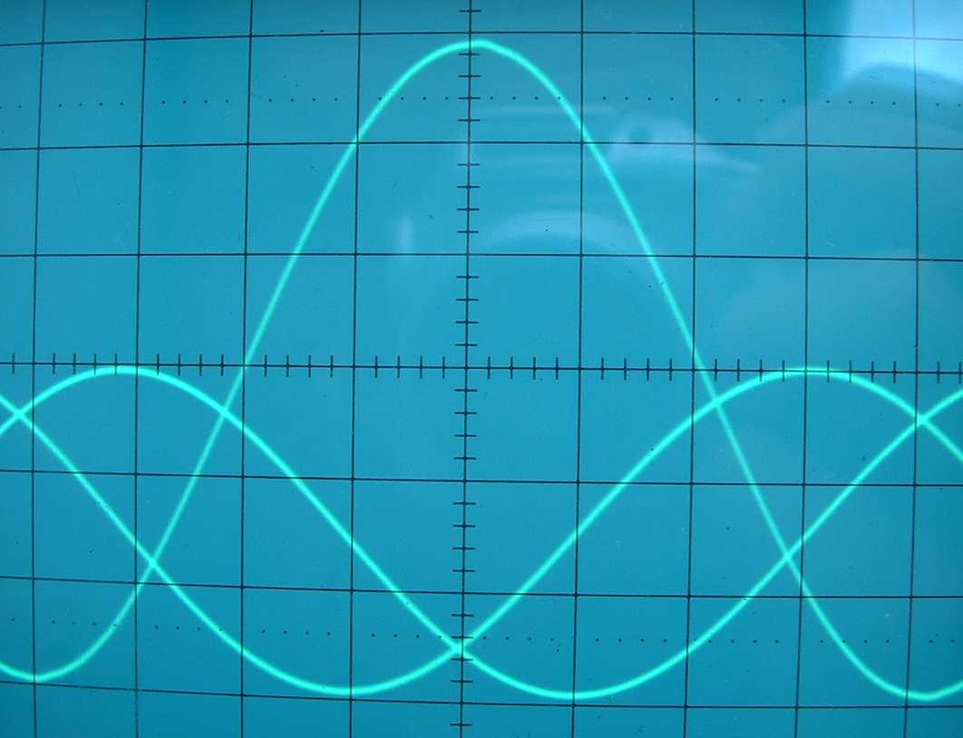 |
| Initial 80 Meter Phasing | Final 80 Meter Phasing |
Reading from the scope, the initial 80 meter current magnitudes are 3.8 : 6.6 : 2.4, and the current phases are -160 : 0 : +154. I am reading from right to left in order to describe the front/director then center then rear/reflector legs. The current magnitudes can be normalized by dividing by 2.4. In that case, the ratios are: 1.58 : 2.75 : 1. The design goal is a ratio of 1 : 2 : 1, and phasing of -140 : 0 : +140. So, we are close, but not close enough.
On top of the current errors, the impedance at the feedpoint was not 50 Ohms. After tweaking, I arrived at the picture on the right. The current magnitudes and phases have been beaten into submission.
On 80 meters, the desired front and rear leg phasing deviation from the center leg is 140 degrees. This value influenced how I set the horizontal time base. I used 4 divisions to span 180 degrees. This means that every division is 45 degrees, and three divisions are 135 degrees, very close to the target of 140 degrees. So, I know that my phase separation is 140 degrees when a trace peaks just a little to the outside of the third division from the center. Each tick is equal to 9 degrees (45 / 5), so 140 degrees, more precisely, would be 3 divisions and 1/2 of a tick from the center (which is 0 degrees).
Let's say that I decided not to tweak the network. What would be the impact on the array performance? Here's where I insert the current numbers back into EZNEC and let it tell me what would happen. The following two response plots show the initial and final responses, going from left to right. These azimuth response plots are made at the take-off angle of maximum gain, which is 21 degrees.
 |
 |
| Initial Phasing Network Azimuth Response | Final Phasing Network Azimuth Response |
Consider the maximum gain, the RDF, and the sharpness of the nulls. The final phasing gain is only 0.4 dB higher. The RDF difference is 0.3 dB, again favoring the final network. Computing the RDF requires the average gain which is not shown on these pictures. The null sharpness can be evaluated visually. At this take-off angle, the deepest initial phasing nulls are slightly more than 15 dB (below the maximum gain). With the final phasing, the nulls deepen to approximately 35 dB. Interestingly, the initial phasing beamwidth is 6.8 degrees narrower.
Unless you care about the deep nulls, and can make use of them, both initial and final networks offer very similar performance. As I said at the start of this page, one of the main reasons to tweak the network is because it's there. It's the challenge of building the paper design, and getting as close as you can to it. One advantage of the final network not apparent in these pattern plots is that the array should have a much wider useful bandwidth. Any excursion from the target frequency will cause the pattern to degrade. When the currents start off degraded, they will become unacceptable with a smaller frequency change.
In the end, if it is impossible to achieve the desired phase relationship and an SWR of 1.0, I will prefer achieving the target phasing. Then, a simple L network can be added to transform the impedance that should have been 50 Ohms to an actual 50 Ohms. Although an L network is two (additional) components, one of the two can usually be combined into the remainder of the network by use of the standard series and parallel combining techniques. This is a compromise in the purity of the Gehrke approach, but the result is correct.
The multiple trace oscilloscope is my primary tool used to measure array phasing. Combined with homemade current probes, coax, and an RF generator, I have a useful test environment. I would never consider an array complete unless I measured its currents. This is a desirable step in a long process, and it verifies the intended performance of the array.
After I've done my best with the phasing network at the target frequency, my last measurement step is to vary the frequency around the target and note the current information as well as the SWR. The SWR degradation determines the operational bandwidth of the array. I usually think in terms of the bandwidth between the frequency points where the SWR is 2.0 or less. I feed the current information back into the EZNEC model to get a sense of the antenna pattern as a function of frequency. My experimentally-based information matches what Gehrke notes on page 43 of the October, 1983, Ham Radio article. He writes: Array performance falls apart more rapidly on the low-frequency side of design center than on the high side.
I have used this technique on vertical arrays, and delta loop arrays. There is no reason why it could not be used on any array, so long as the current probe is adapted for the physical constraints. Recently, the SteppIR Yagi has been introduced, and offers good performance across many bands since each element can be dynamically adjusted for length. It would certainly be possible to add current probes to each element, measure the currents, then feed them back into a model of the antenna. This would allow the user to search for length permutations that provide particular performance not otherwise found in the factory presets.
This page describes my approach to measuring and tweaking a phasing network. Only one direction has been considered. Usually, we electrically rotate the array in several directions through the use of relays and a directional control system. When we change directions, what happens to the phasing? That depends upon the symmetry of the array. Ideally, changing directions will not change the phasing. Achieving symmetry is also work, and I've described my experiences on another page.
Back to my Experimentation Page